

An Illustrative Case Of Quantum Advantage
An Illustrative Case Of Quantum Advantage
The Deutsch-Jozsa quantum algorithm in practice

In my last email, I asked you to vote for the type of emails you want to receive: snippets of posts, full posts, or background stories. The result is clear.
59% of you voted for full posts, 23% voted for snippets, and 18% voted for background stories. Thank you for voting!
So, with no further ado, let’s dive into this week’s post. As usual, you can also read it on Medium.
Posts on quantum computing usually start with anecdotal stories of how it will change the world. It is said to perform tasks in a few seconds that classical computers need thousands of years for.
Then, we start looking into it. First, we learn how quantum bits (qubits) are different from classical bits. They are in a state of superposition. Superposition is a complex (as in complex numbers) linear combination of the states 0 and 1. Many like the notion that the qubit is not 0 or 1, but simultaneously, it is 0 and 1. Even though this notion is not correct — or at least imprecise — it vividly illustrates the advantage of quantum algorithms. While classical computers process their tasks sequentially, one at a time, quantum computers do all the steps at once.
In a previous post, we looked at David Deutsch’s algorithm. This quantum algorithm classifies whether a function is constant (always returns the same result) or balanced (returns different results given different inputs) by only looking at it once. By contrast, a classical algorithm would need to look at the function twice.
The ability of quantum algorithms to evaluate different aspects of an input concurrently is astonishing. But the example we used seems overly simple and construed. It does not provide any practical value. Therefore, we now look at a more practical example.
Let’s consider someone gives you a coin and wants you to bet on either heads or tails. Someone approaching you directly with the intent to gamble? This sounds suspicious, doesn’t it?

Before you agree to play, you first want to make sure the coin is not manipulated. Let’s say there are two options. Either, the coin is fair and lands on each side in half of the cases. Or, the coin is tricked and always lands on the same side. The only reliable way of finding out whether the coin is fair is to toss it and see which side it lands on.
Let’s say we test the coin four times. A fair coin would land on either side two times. So, how often do you need to toss the coin to find out? If you toss it only once, it lands either heads-up or tails-up. This tells you nothing at all. If you toss it again and it lands on the other side, you’re done. Then, you know that it is a fair coin. But what if the coin lands on the same side again? A fair coin may land on one side two out of four times. To say for sure that a coin is tricked, you need to toss it at least three times (when we assume that it is fair at a sample size of four).
Mathematically, when the coin is fair at n tosses, we need to toss the coin 2^(n/2–1)+1 times. For n=4, these are 2^(4/2–1)+1=3 tosses. For n=8, these were 2^(8/2–1)+1=7 tosses, for n=10, these were 2^(10/2–1)+1=15 tosses, and so on. This number increases exponentially.
In the worst possible scenario, we could get the same result repeatedly without knowing whether the coin could still be fair. It would require an exponential number of inquiries — at least if we’re doing it classically.
With quantum computing, we can solve this problem in a single run. Instead, we use a qubit for each possible combination of tosses. For simplicity, let’s say we toss the coin only three times. And, let’s say 1 represents heads, and 0 represents tails. Thus, there are eight possible inputs: (0,0,0), (0,0,1), (0,1,0), (0,1,1), (1,0,0), (1,0,1), (1,1,0), (1,1,1).
In our quantum circuit, we use one qubit for each toss we consider, plus one auxiliary qubit. Therefore, we use four qubits.
We start with importing the required libraries and specifying the quantum circuit. The circuit contains a quantum register representing the tosses, a quantum register containing the auxiliary qubit, and a classical register to receive the measurements.
from qiskit import QuantumCircuit, QuantumRegister, ClassicalRegister, Aer, execute
from qiskit.visualization import plot_histogram

TOSSES = 3

qr = QuantumRegister(TOSSES, "toss")
aux = QuantumRegister(1, "aux")
cr = ClassicalRegister(TOSSES, "cr")
qc = QuantumCircuit(qr, aux, cr)
The main part of the algorithm is the quantum oracle. If this is the first time you hear of an oracle in quantum computing, don’t worry. It is not a magic trick, and it does not involve supernatural power. The quantum oracle is nothing but a placeholder for a transformation gate. The oracle is like the switch-case control structure you may know from classical programming. You have a variable, the oracle. And you specify the behavior for each possible value it may have.

In our case, the oracle represents the behavior of the coin. A tricked coin either produces only 0s or only 1s.
Qiskit initializes a qubit in state |0⟩. In this state, we always measure a qubit as 0. So, when we do nothing, we already have the oracle representing a tricked coin that always lands tails up.
We wrap “doing nothing” into a function anyway. This function creates a custom transformation gate for us. To make clear what we do, we apply I-gates on all qubits representing the tosses. The I-gate is the identity gate and leaves the qubit unchanged.
def tails_oracle(qr, aux):
    # Create a sub-circuit
    oc = QuantumCircuit(qr, aux)

    oc.i(qr)

    # We return the oracle as a gate
    oracle = oc.to_gate()
    oracle.name = "tails"
    return oracle
The following figure depicts the tails_oracle graphically.
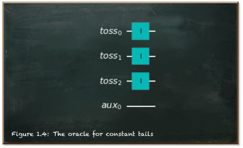
When we run a circuit that consists only of this oracle, it outputs the state 000—representing three times tails-up.

The NOT-gate flips a qubit from state |0⟩ to state |1⟩. Therefore, we can create the oracle representing a tricked coin that always lands heads-up by applying NOT-gates to all qubits.
def heads_oracle(qr, aux):
    # Create a sub-circuit
    oc = QuantumCircuit(qr, aux)

    oc.x(qr)

    # We return the oracle as a gate
    oracle = oc.to_gate()
    oracle.name = "heads"
    return oracle
The following figure depicts this oracle.
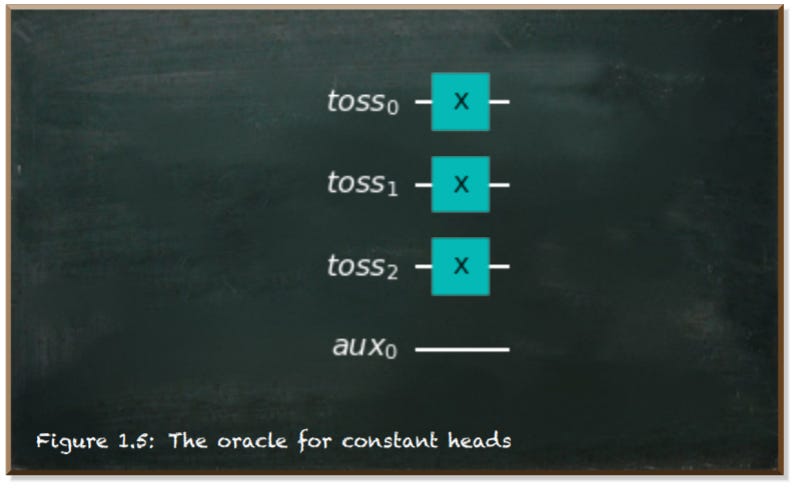
This oracle always produces the state 111— the state representing three times heads-up.
The oracle representing a fair coin is a little trickier. Though, it is not too complex either. With three qubits, we can say that it lands at least once heads-up and once tails-up. The function balanced_oracle takes the additional config parameter. This is supposed to be a bit string that represents the outcome of tossing the coin. We apply NOT-gates to the qubits that represent a heads-up toss.
Furthermore, we add controlled-NOT gates with each toss as the control qubit and the auxiliary as the target qubit.
def balanced_oracle(qr, aux, config):
    # Create a sub-circuit
    oc = QuantumCircuit(qr, aux)

    for pos in range(len(config)):
        if config[pos] == '1':
            oc.x(qr[pos])

        oc.cx(qr[pos], aux)

    # We return the oracle as a gate
    oracle = oc.to_gate()
    oracle.name = "balanced"
    return oracle
The following figure depicts the balanced oracle for the configuration 110— standing for heads-heads-tails.
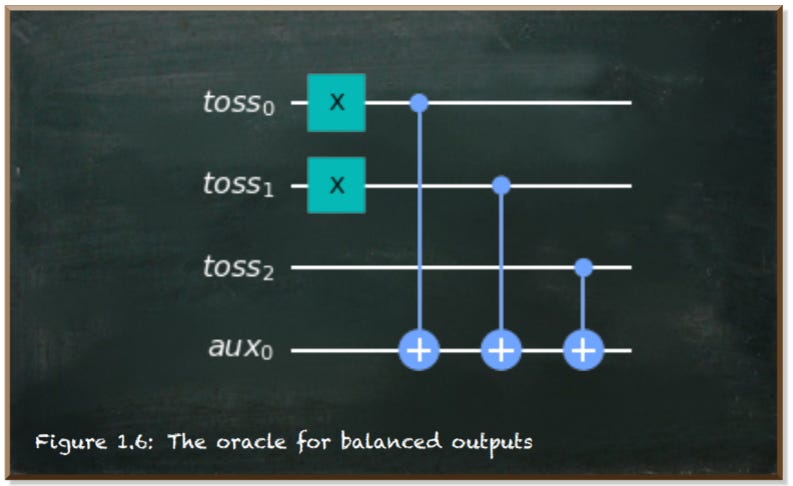
This oracle results in the state we specify in the config bit string. In our example, it is 110. It works for all other inputs, too. Note that the qubits read from right to left.

Apparently, the three CNOT-gates did not affect. It seems plausible since the CNOT-gate acts like a NOT-gate applied on the target qubit only if the control qubit is in state |1⟩. And all our qubits are in state |0⟩. See this post for a more detailed view of the CNOT-gate.
The question arises: “If the CNOT-gate don’t matter, why do we add them in the first place?”
The answer is our quantum algorithm. Thus far, we have only created the oracles for different situations. We saw that the oracles correctly represent the behavior of the coin.
So, let’s implement our algorithm that identifies whether the coin is constant (tricked) or balanced (fair).
We start with a series of Hadamard gates to bring the qubits into state |+⟩ and the auxiliary qubit into state |-⟩. In these states, a qubit has the probability of being measured as 0 or as 1 of 50% each. The difference between state |+⟩ and state |-⟩ is the qubit phase (see this post to learn more about the qubit phase).
Then, we apply the oracle. Finally, we apply another Hadamard gate on the qubits to bring them back from superposition into a basis state.
qr = QuantumRegister(TOSSES, "toss")
aux = QuantumRegister(1, "aux")
cr = ClassicalRegister(TOSSES, "cr")
qc = QuantumCircuit(qr, aux, cr)

# Bring the qubits into superposition, state |+>
qc.h(qr)

# Bring the auxiliary qubit into state |->
qc.x(aux)
qc.h(aux)

# Apply the oracle
# ...

# Bring the qubits back to a basis state
qc.h(qr)

# measure the qubits
qc.measure(qr, cr)
The following image shows the circuit, including an oracle.
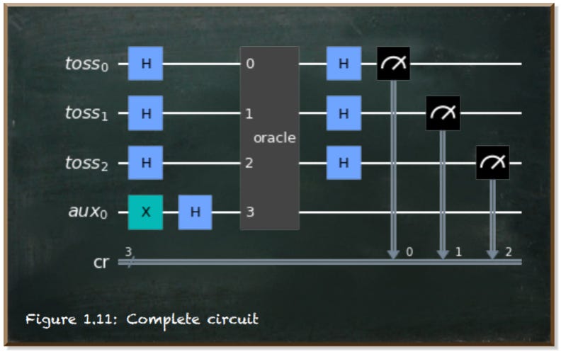
So. let’s see this circuit in action. We start with the oracle for the constant tails-up coin.
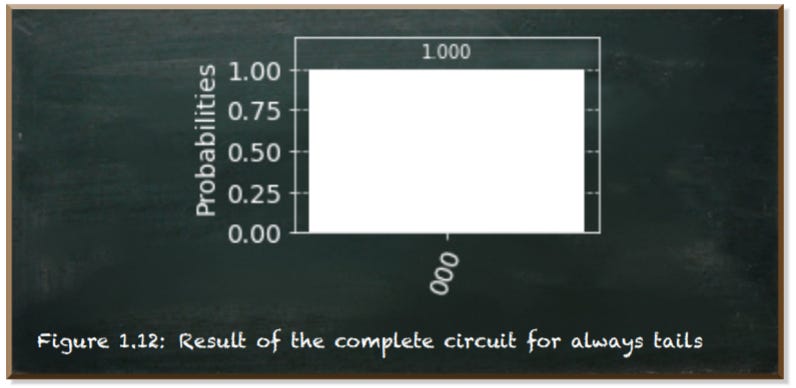
It ends up in state 000.
Next, we run the algorithm with the heads_oracle.

It also ends up in state 000.
Finally, we run the circuit with the balanced oracle (you can run it with any bitstring).
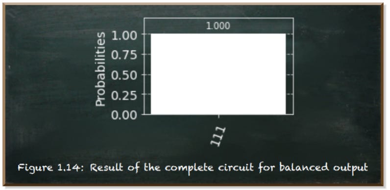
With the oracle for balanced input, the circuit ends up in state 111. It doesn’t matter which bit string you provide as input.
“But how does this work?”
When the oracle is constant, we either apply I-gates or NOT-gates. But since our algorithm puts the qubits into state |+⟩, we do not change anything. When we apply the NOT-gate on a qubit in state |+⟩, it stays in that state. When we apply the Hadamard-gates at the end of our circuit, they turn the qubits from state |+⟩ back into state |0⟩. We have simple HIH sequences.
But when we apply the balanced_oracle, we additionally apply CNOT-gates. While these do not matter if the qubits are in a basis state (such as |0⟩), they do matter if the qubit is in superposition. Then, the CNOT-gate applies the phase of the target qubit on the control qubit. We use the auxiliary qubit as the target qubit in our circuit, and we put it into state |-⟩. So, when we apply the CNOT-gates, we “copy” this phase onto the other qubits.
As a result, these qubits are switched to state |-⟩, too. The final Hadamard gates turn qubits in state |-⟩ into state |1⟩. We call this effect phase kickback.
Conclusion
developed this algorithm. It is a generalization of Deutsch’s algorithm that works with only two qubits.
This algorithm is one of the first examples of a quantum algorithm exponentially faster than a classical algorithm.
Furthermore, an algorithm uses quite a few quantum-specific techniques, such as superposition, oracles, and phase kickback. And, when you work through these techniques step by step, you get a pretty good feeling of how quantum algorithms work in practice.
You're interested in quantum computing and machine learning...
...But you don't know how to get started?
