

How To Create Quantum Multinoulli Distributions With Qiskit
How To Create Quantum Multinoulli Distributions With Qiskit
Quantum machine learning in practice

You can read this post on Medium.
Probability distributions are ubiquitous in machine learning. It doesn't matter whether we aim to answer the simplest question or solve the biggest problem. Technically, the goal always is to learn a yet unknown probability distribution from data.
It doesn't matter if we do a simple regression analysis or train a deep neural network, either. The goal always is to find that certain probability distribution.
And, it doesn't even matter if you use quantum machine learning algorithms. In the end, the answer you're looking for will be probabilistic.
But not all probability distributions are alike. They can be pretty heterogeneous. And each type of distribution has its specificities you'd better know. You're in trouble if you don't know what kind of distribution fits your problem at hand.
Furthermore, you are not better off if you know which distribution fits your problem but don't know how to generate an appropriate distribution. And, guess what, generating distributions with qubits is a challenge in itself.
Classical computers have billions of bits of memory. Sparing a few to store a probability distribution is no big deal. But a quantum computer has less than a hundred qubits. We should think about how we can represent a probability distribution efficiently. Fortunately, a qubit is not just 0 or 1. Even though it is only 0 or 1 if we measure it, it is in a quantum state of superposition. And this state contains a lot more information.
Previously, we looked at how to create a quantum system that reproduces a Bernoulli distribution. The Bernoulli distribution is the simplest of all. There are only two possible values, each occurring with a certain probability. That's pretty much what the superposition of a single qubit denotes.
Let's say our single qubit is in state |𝜓⟩=√0.7|0⟩+√0.3|1⟩. If you measure many qubits in this state, it results in the following Bernoulli distribution.
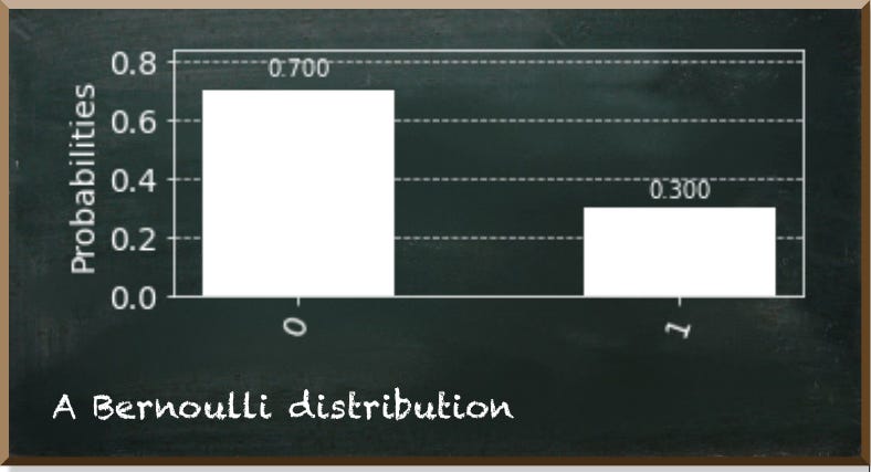
The Bernoulli distribution answers simple questions you could answer with yes or no. For instance, did a passenger survive the Titanic shipwreck? Is this a cat? Does the student pass the exam?
But what if we have multiple possible answers? Let's say we want to label handwritten digits from the famous MNIST dataset? Apparently, we need to distinguish between more than two output values.
We need multiple qubits to represent all categories, for we measure a single qubit as 0 or 1. Let's say we want to label the digits from 0 to 7. Then, we have eight different categories. We could encode these possible outcomes with three qubits. Each combination of the qubit measurements represents a number. 000 represents the digit 0. 001 represents 1. 010 represents 2. 011 represents 3, and so on. Finally, 111 represents 7.
As a result, we would get a Multinoulli distribution, also called the categorical distribution. It covers the case where an event will have one of multiple possible outcomes. Therefore, it generalizes the Bernoulli distribution that covers events with one out of precisely two possible outcomes.
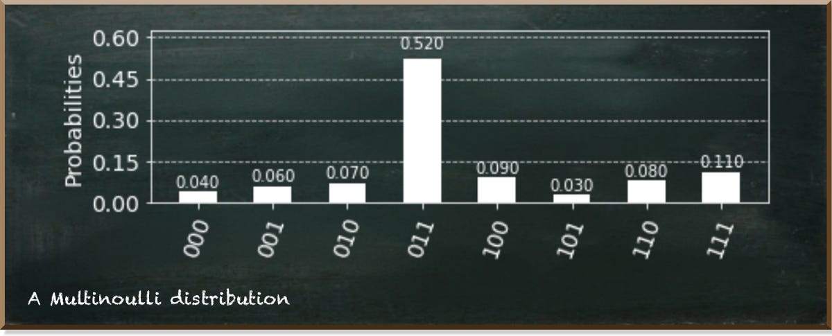
So, let's say we have the following data of such a Multinoulli distribution
dist = {
    '000': 0.04, # 0
    '001': 0.06, # 1
    '010': 0.07, # 2
    '011': 0.52, # 3
    '100': 0.09, # 4
    '101': 0.03, # 5
    '110': 0.08, # 6
    '111': 0.11, # 7
}
The practical question is: "How can we let a quantum circuit represent such a distribution?"
The easiest method is to transform these probabilities into amplitudes and pass them to the initialize function of the quantum circuit.
from qiskit import QuantumCircuit, Aer, execute
from qiskit.visualization import plot_histogram
from math import sqrt

qc = QuantumCircuit(3)
initial_state = list(map(lambda x: sqrt(x), dist.values()))
qc.initialize(initial_state)

results = execute(qc,
  Aer.get_backend('statevector_simulator')
).result().get_counts()
plot_histogram(results)
The real magic happens in line 6. We compute the initial state of our three-qubit system. The whole trick is to take the square root of each probability because the probability is the square of a quantum state amplitude.
The initialize function of the Qiskit QuantumCircuit takes a list of all amplitudes as an input parameter (see the official Qiskit documentation).
When we execute this circuit with the 'statevector_simulator', it reproduces the exact distribution we specified.
Is there another way? Could we create a Multinoulli distribution by using quantum gates?
Of course. But, it is not as straightforward.
We can use quantum gates to transform the state of qubits. For instance, we can use the qc.ry(theta, 0) function to rotate the state vector of the qubit at position 0 by the angle theta. Moreover, we can calculate the angle theta from a probability using a prob_to_angle function. Have a look at this post for further details.
The problem is that we use the value of a single qubit for different values in our distribution. For instance, the left-digit is 1 for all the states ['100', '101', '110', '111'].
So, when we specify the state of qubit 3 (the qubit at the left-hand side), we need to take the sum of the probabilities of all these states.
from qiskit import QuantumRegister

def prob_to_angle(prob):
    return 2*asin(sqrt(prob))

qr = QuantumRegister(3)
qc = QuantumCircuit(qr)

range_4_to_7 = list(filter (lambda item: item[0][0] == "1", dist.items()))
sum_4_to_7 = sum(map(lambda item: item[1], range_4_to_7))

qc.ry(prob_to_angle(sum_4_to_7),2)
First, we define our convenience function prob_to_angle and define a QuantumRegister. The QuantumRegister is a container for our qubits that allows us to address single qubits easily in our Python code.
The action starts in line 9. There, we separate the values of our distribution from four to seven, calculate the sum of these states, and split our overall probability into halves. The following figure depicts the state thus far.
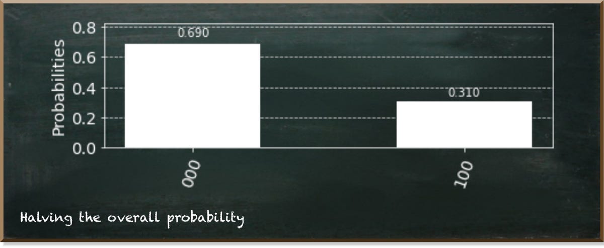
As a result, we distinguish only two groups of states. Those where the upper qubit is 0 and those where it is 1. (Note: the upper qubit is at the left-hand, lower side of the string in the figure.)
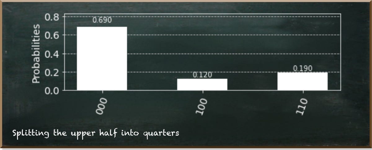
In the next step, we further halve the second half. We apply the same logic. We split the states where the upper qubit is 1 into two quarters.
range_6_to_7 = list(filter (lambda item: item[0][1] == "1", range_4_to_7))
sum_6_to_7 = sum(map(lambda item: item[1], range_6_to_7))

qc.cry(prob_to_angle(sum_6_to_7/sum_4_to_7),2,1)
The only difference to the first split is the quantum gate we use. This time, we use the controlled RY gate instead of the plain RY gate. The difference is that the controlled RY gate only applies the split of probabilities if the control qubit is 1. In our case, this means that we only split the 100 block and left the 000 block untouched.
Finally, we need one more split of the upper quarters. We have to take care of each quarter separately. First, we split the upper quarter into two halves. Now, we must only touch the state where the two upper qubits are 1. Therefore, we use the multi-controlled RY gate (qc.mcry).
At this point, the QuantumRegister comes in handy because we can access the qubits as an array. The term qr[1:] selects all qubits except the first. These are the control qubits for the multi-controlled RY gate. The last argument qr[0] denotes the target qubit.
qc.mcry(prob_to_angle(dist['111']/sum_6_to_7),qr[1:],qr[0])
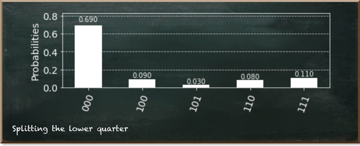
range_4_to_5 = list(filter (lambda item: item[0][1] == "0", range_4_to_7))
sum_4_to_5 = sum(map(lambda item: item[1], range_4_to_5))
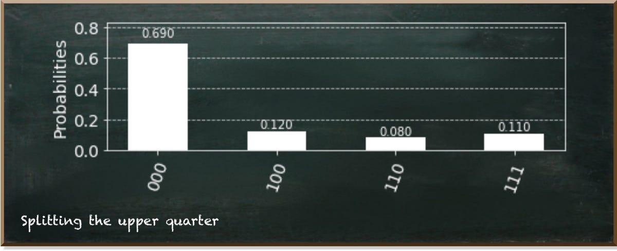
We also need to split the lower quarter using another multi-controlled RY gate. We encapsulate it into NOT gates that we apply on the middle qubit. This lets us select the states where the middle qubit is 0 instead of 1.
qc.x(1)
qc.mcry(prob_to_angle(dist['101']/sum_4_to_5),qr[1:],qr[0])
qc.x(1)
The result so far shows that we prepared half of the states.
We also need to perform the corresponding steps on the lower half to produce the overall distribution. Here's the complete source code.
def prob_to_angle(prob):
    return 2*asin(sqrt(prob))

qr = QuantumRegister(3)
qc = QuantumCircuit(qr)

# split into halves, work with the upper half
range_4_to_7 = list(filter (lambda item: item[0][0] == "1", dist.items()))
sum_4_to_7 = sum(map(lambda item: item[1], range_4_to_7))

qc.ry(prob_to_angle(sum_4_to_7),2)

# split upper half into quarters, work with the upper quarter
range_6_to_7 = list(filter (lambda item: item[0][1] == "1", range_4_to_7))
sum_6_to_7 = sum(map(lambda item: item[1], range_6_to_7))

qc.cry(prob_to_angle(sum_6_to_7/sum_4_to_7),2,1)

# change upper qubit
qc.mcry(prob_to_angle(dist['111']/sum_6_to_7),qr[1:],qr[0])

# work with lower quarter of upper half
qc.x(1)

range_4_to_5 = list(filter (lambda item: item[0][1] == "0", range_4_to_7))
sum_4_to_5 = sum(map(lambda item: item[1], range_4_to_5))

qc.mcry(prob_to_angle(dist['101']/sum_4_to_5),qr[1:],qr[0])
qc.x(1)

# work with lower half
range_0_to_3 = list(filter (lambda item: item[0][0] == "0", dist.items()))
sum_0_to_3 = sum(map(lambda item: item[1], range_0_to_3))
qc.x(2)

# split lower half into quarters, work with the upper quarter
range_2_to_3 = list(filter (lambda item: item[0][1] == "1", range_0_to_3))
sum_2_to_3 = sum(map(lambda item: item[1], range_2_to_3))

qc.cry(prob_to_angle(sum_2_to_3/sum_0_to_3),2,1)

# change upper qubit
qc.mcry(prob_to_angle(dist['011']/sum_2_to_3),qr[1:],qr[0])

# work with lower quarter of upper half
qc.x(1)

range_0_to_1 = list(filter (lambda item: item[0][1] == "0", range_0_to_3))
sum_0_to_1 = sum(map(lambda item: item[1], range_0_to_1))

qc.mcry(prob_to_angle(dist['001']/sum_0_to_1),qr[1:],qr[0])
qc.x(1)

# unselect the lower half
qc.x(2)

results = execute(qc,Aer.get_backend('statevector_simulator')).result().get_counts()
plot_histogram(results)
When we look at the result, we see that it resembles our Multinoulli distribution.
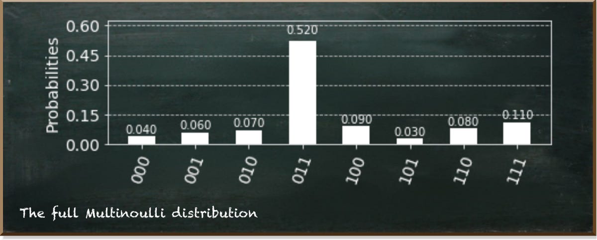
The approach is straightforward. We repeatedly split the states into halves and apply the corresponding qubit transformation. However, it is a lot more code than simply initializing the three qubits with the probabilities.
But in some situations, you won't be able to specify all the probabilities during initialization. For instance, if you create a Quantum Bayesian Network, the distribution values may result from other variables. Then, you inevitably want to be able to create a Multinoulli distribution programmatically.
You're interested in quantum computing and machine learning...
...But you don't know how to get started?
