

Practically Exploring The Axioms Of Quantum Computing
Practically Exploring The Axioms Of Quantum Computing
Towards quantum computing mastery

You can read this post on Medium.
On your way towards quantum computing mastery, you’ll encounter a lot of weird phenomena. Just take the quantum superposition, for instance. It says a quantum bit (qubit) is in a complex linear combination of 0 and 1.
If you’re a mathematician or a physicist, you’ll value when someone uses a correct definition of such a term. But if you’re not, you’ll likely prefer a more anecdotal explanation, such as the qubit is 0 and 1 concurrently.
As a non-mathematician, you seem doomed either way. The correct definition is as good as a set of hieroglyphs. But, the anecdotal explanation is simply wrong.

But there’s a third way: the practical way. Quantum computing is no longer a theoretical construct. There are real quantum computers. And, even if you don’t have access to them, there are quantum SDKs, like Qiskit, that contain simulators. You can develop and run quantum circuits on your local computer. Of course, you won’t see any quantum speedup if you use a classical computer. But it is good enough to learn quantum computing in a practical hands-on manner.
So, let’s look at a qubit. This piece of code creates a quantum circuit with a single qubit. Then, it executes the circuit and outputs the Bloch Sphere.
from qiskit import QuantumCircuit, Aer, execute
from qiskit.visualization import plot_bloch_multivector

qc = QuantumCircuit(1)

out = execute(qc,Aer.get_backend('statevector_simulator')).result().get_statevector()
plot_bloch_multivector(out)
The Bloch Sphere is a widely used representation of the qubit. It prominently shows the two basis states of the qubit at the poles of the sphere. More specifically, qubit states are represented by vectors from the center of the sphere to its surface. The two basis vectors end at the poles.
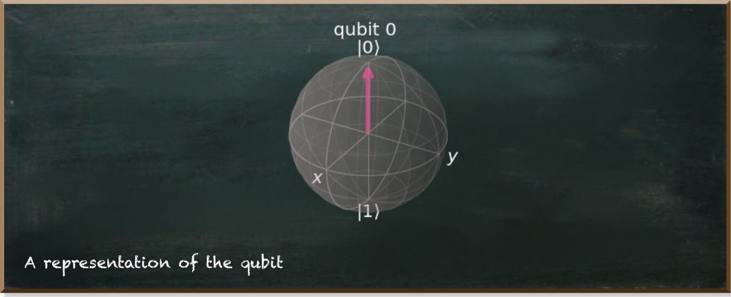
Our figure shows the vector |0⟩ that ends at the north pole. |0⟩ is nothing fancy. But it is simply the (Dirac) notation we use in quantum mechanics to describe vectors.
In general, the vector |0⟩ is not exceptional. However, practically, we use it as a computational basis. That means if we measure a qubit in state |0⟩, we will always observe it as 0. Let’s do this practically.
from qiskit import QuantumCircuit, Aer, execute
from qiskit.visualization import plot_histogram
qc = QuantumCircuit(1)
qc.measure_all()
results = execute(qc,Aer.get_backend('qasm_simulator')).result().get_counts()
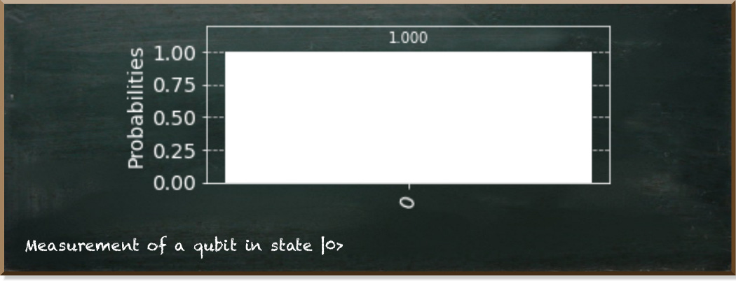
plot_histogram(results, figsize=(5,2), color=['white'])The following figure depicts the output of the code above. It shows the probabilities of all possible measurements. In our case, there is only one possible outcome: 0.
As mentioned, the qubit has two basis states. The second basis state is |1⟩ that we measure as 1.
from qiskit import QuantumCircuit, Aer, execute
from qiskit.visualization import plot_histogram

qc = QuantumCircuit(1)
qc.x(0)
qc.measure_all()

results = execute(qc,Aer.get_backend('qasm_simulator')).result().get_counts()
plot_histogram(results, figsize=(5,2), color=['white'])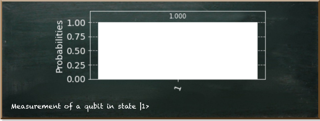
When we look at the vector |1⟩ in the Bloch Sphere, we see it points south.

Limiting our qubits to these two basis states is as good (or simple) as regular bits. But, of course, to use the advantage of qubits, we must allow them to be in other states, too.
|+⟩ is one of these states. We reach this state by rotating the qubit state vector by 𝜋/2 around the Y-axis. In this state, the qubit has the same probability of being 0 or 1–50% each.
from qiskit import QuantumCircuit, Aer, execute
from qiskit.visualization import plot_histogram
from math import pi

qc = QuantumCircuit(1)
qc.ry(pi/2, 0)

results = execute(qc,Aer.get_backend('statevector_simulator')).result().get_counts()
plot_histogram(results, figsize=(5,2), color=['white'])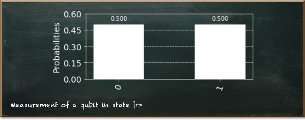
When we look at the Bloch Sphere, we see that it ends at the X-axis on the sphere's equator. So, graphically, the distance to either one pole is the same.

Something similar happens if we rotate the vector |1⟩ by 𝜋/2 around the Y-axis. It results in state |−⟩.
from qiskit import QuantumCircuit, Aer, execute
from qiskit.visualization import plot_histogram
from math import pi

qc = QuantumCircuit(1)
qc.x(0)
qc.ry(pi/2, 0)

out = execute(qc,Aer.get_backend('statevector_simulator')).result().get_statevector()
plot_bloch_multivector(out)
The resulting vector resides at the X-axis, too. Therefore, when we measure the qubit, it has the same probability of being 0 or 1.

Practically, you may think that states |+⟩ and |−⟩ are the same. This couldn’t be farther from the truth. By contrast, as the visual representations of the Bloch Spheres show, these two states point in opposite directions.
In quantum mechanical terms, they are mutually orthogonal to each other. This means that we can clearly distinguish one from another. It may sound weird. How can we determine two states that exhibit the same measurement probabilities?
To answer this question, we need to clarify an essential aspect. The quantum state only exists as long as we don’t measure the qubit. But once we measure it, it instantly jumps to one of the two basis states. But nobody dictates us to leave the qubits precisely as they are before we measure them. In fact, one of the most important parts of quantum computing is to change the quantum system so that two different states result in two different measurements.
In the case of |+⟩ and |−⟩, we can rotate them back around the Y-axis before measuring them. Of course, we know that we rotated the qubit back. Then, if we measure 0, we can deduce that the qubit must have been in state |+⟩. And, we know that it must have been in state |−⟩ if we measured 1.
Only if quantum states are mutually orthogonal to each other can we tell them apart with certainty. But we can’t otherwise. So, for instance, let’s say someone hands you a single qubit that is either in state |0⟩ or state |+⟩. How do you decide which one it is?
If you measure it right away, you may be lucky to measure 1. Then, you know that it must have been in state |+⟩ because you never observe a qubit as 1 in state |0⟩. But your chances to be lucky are 50%. If you measure 0, the qubit’s state could have been |0⟩ or |+⟩.
The best you can do is to rotate the by 𝜋/4. If the qubit were in state |0⟩, you’d get an 85% chance of measuring it as 0.
from qiskit import QuantumCircuit, Aer, execute
from qiskit.visualization import plot_bloch_multivector

# a qubit in state |0>
qc = QuantumCircuit(1)

# Rotate the qubit
qc.ry(pi/4, 0)

results = execute(qc,Aer.get_backend('statevector_simulator')).result().get_counts()
plot_histogram(results, figsize=(5,2), color=['white'])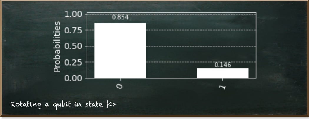
Respectively, if the qubit was in state |+⟩, you see the reversed probability of measuring it as 1.
from qiskit import QuantumCircuit, Aer, execute
from qiskit.visualization import plot_bloch_multivector

# put qubit into state |+>
qc = QuantumCircuit(1)
qc.ry(pi/2, 0)

# Rotate the qubit
qc.ry(pi/4, 0)

results = execute(qc,Aer.get_backend('statevector_simulator')).result().get_counts()
plot_histogram(results, figsize=(5,2), color=['white'])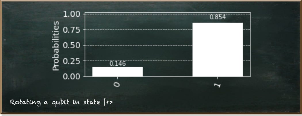
In the end, the result you get is probabilistic. You can’t say with absolute certainty whether the qubit was in state |0⟩ or |+⟩.
You are only able to distinguish qubit states clearly if they are mutually orthogonal. But this is not the usual case. Especially not if you create quantum algorithms that exhibit a significant speedup.
You're interested in quantum computing and machine learning...
...But you don't know how to get started?
