Quantum Measurement Mitigation With Qiskit

The next step toward participating in IBM's Quantum Open Science Prize

The submission deadline for IBM’s Quantum Open Science Prize is this week! If you want to participate, please hurry. In today’s post, we will do a big step toward sending in our submission. But there are still a few steps ahead of us.

Don’t worry. First, I will keep posting the missing steps. Second, in case you need the remaining steps for your own submission, you can already access them.

You find all steps in my GitHub repository. Furthermore, you can also have a look at my submission. I don’t want to spoil too much, but, we reached the entry criteria!

---

Today, we're implementing a quantum measurement error mitigation method with Qiskit. We do this to participate in IBM's second Quantum Open Science Prize. They ask for a solution to a quantum simulation problem. They want us to simulate a Heisenberg model Hamiltonian for a three-particle system on their 7-qubit Jakarta system using Trotterization. The hard part is not to simulate a Heisenberg model Hamiltonian. It is not a problem to do it for a three-particle system, either. And, using Trotterization is — yes, that's right — no problem, too.

Surprisingly, the problem is doing all this on an actual 7-qubit device. Quantum systems are incredibly fragile. They are susceptible to environmental disturbances and prone to errors. Unfortunately, we don't have the resources (yet) to correct these errors on hardware or low software level. The best we can do is reduce the noise's effects on the computation.

Luckily, there are quite a few quantum error mitigation methods out there. In previous posts, we closely looked at the Clifford Data Regression (CDR) method. We even used it to reduce the noise in a simulation and on an actual quantum device(https://towardsdatascience.com/practical-error-mitigation-on-a-real-quantum-computer-41a99dddf740).

The CDR reduces the noise when calculating the expectation value of an observable. But to participate in IBM's challenge, we need to reduce errors in the measurement counts. IBM uses a quantum state tomography algorithm to calculate how closely the resulting state matches the expected state. And this algorithm works with the measurement counts.

Unfortunately, while we can calculate the expectation value from the counts, we can't do it the other way around. So instead, we need to adapt our quantum error mitigation methods to work with the measurement counts. In other words, we're implementing a quantum measurement error mitigation.

Did I say that simulating a Heisenberg model Hamiltonian for a three-particle system using Trotterization is not a problem? I am a man of my word. The following source code provides the required simulation. IBM provides this code as part of their exemplary GitHub project.

There's only one change. If we set the variable measure to True we append a ClassicalRegister to the circuit to receive the measurements.

measure = True

# Trotterized circuit from IBM material
from qiskit.circuit import Parameter
from qiskit import QuantumCircuit, QuantumRegister, ClassicalRegister

# YOUR TROTTERIZATION GOES HERE -- START (beginning of example)

# Parameterize variable t to be evaluated at t=pi later
t = Parameter('t')

# Build a subcircuit for XX(t) two-qubit gate
XX_qr = QuantumRegister(2)
XX_qc = QuantumCircuit(XX_qr, name='XX')

XX_qc.ry(np.pi/2,[0,1])
XX_qc.cnot(0,1)
XX_qc.rz(2 * t, 1)
XX_qc.cnot(0,1)
XX_qc.ry(-np.pi/2,[0,1])

# Convert custom quantum circuit into a gate
XX = XX_qc.to_instruction()

# Build a subcircuit for YY(t) two-qubit gate
YY_qr = QuantumRegister(2)
YY_qc = QuantumCircuit(YY_qr, name='YY')

YY_qc.rx(np.pi/2,[0,1])
YY_qc.cnot(0,1)
YY_qc.rz(2 * t, 1)
YY_qc.cnot(0,1)
YY_qc.rx(-np.pi/2,[0,1])

# Convert custom quantum circuit into a gate
YY = YY_qc.to_instruction()

# Build a subcircuit for ZZ(t) two-qubit gate
ZZ_qr = QuantumRegister(2)
ZZ_qc = QuantumCircuit(ZZ_qr, name='ZZ')

ZZ_qc.cnot(0,1)
ZZ_qc.rz(2 * t, 1)
ZZ_qc.cnot(0,1)

# Convert custom quantum circuit into a gate
ZZ = ZZ_qc.to_instruction()

# Combine subcircuits into a single multiqubit gate representing a single trotter step
num_qubits = 3

Trot_qr = QuantumRegister(num_qubits)
Trot_qc = QuantumCircuit(Trot_qr, name='Trot')

for i in range(0, num_qubits - 1):
    Trot_qc.append(ZZ, [Trot_qr[i], Trot_qr[i+1]])
    Trot_qc.append(YY, [Trot_qr[i], Trot_qr[i+1]])
    Trot_qc.append(XX, [Trot_qr[i], Trot_qr[i+1]])

# Convert custom quantum circuit into a gate
Trot_gate = Trot_qc.to_instruction()
XX_qc.draw()
# YOUR TROTTERIZATION GOES HERE -- FINISH (end of example)


# The final time of the state evolution
target_time = np.pi

# Number of trotter steps
trotter_steps = 8  ### CAN BE >= 4

# Initialize quantum circuit for 3 qubits
qr = QuantumRegister(7)
cr = ClassicalRegister(3)
qc = QuantumCircuit(qr, cr) if measure is True else QuantumCircuit(qr)

# Prepare initial state (remember we are only evolving 3 of the 7 qubits on jakarta qubits (q_5, q_3, q_1) corresponding to the state |110>)
qc.x([3,5])  # DO NOT MODIFY (|q_5,q_3,q_1> = |110>)

# Simulate time evolution under H_heis3 Hamiltonian
for _ in range(trotter_steps):
    qc.append(Trot_gate, [qr[1], qr[3], qr[5]])

# Evaluate simulation at target_time (t=pi) meaning each trotter step evolves pi/trotter_steps in time
qc = qc.bind_parameters({t: target_time/trotter_steps})

Today, we want to focus on measurement mitigation. Thus, we take the code as it is. We end up with qc as our quantum circuit.

The following figure depicts the circuit diagram.

Next, we need a runtime environment. Today we are ok with simulated environments. But to be as close as possible to a real quantum computer, we load the noise signature from a real device. We connect to our IBM account and obtain the Jakarta backend from it for that purpose. [This post](https://towardsdatascience.com/how-to-run-code-on-a-real-quantum-computer-c1fc61ff5b4) elaborates on how you can get the free IBM account if you don't have one yet.

In fact, we need two environments. Next to the noisy simulator, we need a noise-free environment. The Qiskit QasmSimulator does that job for us.

# IBM account 
from qiskit.providers.aer import QasmSimulator

# load IBMQ Account data
from qiskit import IBMQ

# replace TOKEN with your API token string (https://quantum-computing.ibm.com/lab/docs/iql/manage/account/ibmq)
IBMQ.save_account("TOKEN", overwrite=True) 
account = IBMQ.load_account()

provider = IBMQ.get_provider(hub='ibm-q-community', group='ibmquantumawards', project='open-science-22')
jakarta = provider.get_backend('ibmq_jakarta')

# Simulated backend based on ibmq_jakarta's device noise profile
sim_noisy_jakarta = QasmSimulator.from_backend(provider.get_backend('ibmq_jakarta'))

# Noiseless simulated backend
sim = QasmSimulator()

Let's now run our quantum circuit with both simulators.

from qiskit import assemble, execute, transpile, Aer

shots = 1024

qc.measure([1,3,5], cr)

t_qc = transpile(qc, sim_noisy_jakarta)
qobj = assemble(t_qc)
counts = sim_noisy_jakarta.run(qobj, shots=shots).result().get_counts()

t_qc_sim = transpile(qc, sim)
noiseless_result = sim.run(assemble(t_qc_sim), shots=shots).result()
noiseless_counts = noiseless_result.get_counts()
    
print("noisy:      ", counts)
print("noise-free: ", noiseless_counts)

noisy:       {'101': 106, '111': 124, '011': 141, '000': 113, '010': 124, '100': 115, '110': 207, '001': 94}
noise-free:  {'101': 34, '110': 866, '011': 124}

The counts differ significantly. So, let's remove the noise! We can calculate a modifier that turns the noisy value into a noise-free for each state.

For instance, we observed the state |101⟩ 105 times in the noisy simulation but only 30 times in the noise-free. We get the noise-free value when we multiply the noisy value by the modifier 30/105.

Let's do this for all eight states.

from collections import Counter
from functools import reduce

def sorted_counts(counts):
    complete = dict(reduce(lambda a, b: a.update(b) or a, [{'000': 0, '001': 0, '010': 0, '011': 0, '100': 0, '101': 0, '110': 0, '111': 0}, counts], Counter()))
    return {k: v for k, v in sorted(complete.items(), key=lambda item: item[0])}


zipped = list(zip(sorted_counts(noiseless_counts).values(), sorted_counts(counts).values()))
modifier = list(map(lambda pair: pair[0]/pair[1], zipped))

print("modifier: ", modifier)

modifier:  [0.0, 0.0, 0.0, 0.8794326241134752, 0.0, 0.32075471698113206, 4.183574879227053, 0.0]

First, we add a small helper function sorted_counts. It does two things. On the one hand, it makes sure that all state keys exist. For instance, the key 000 representing state |000⟩ doesn't exist in the noise-free counts. On the other hand, the function sorts the counts by their key, starting with 000 and ending with 111.

This is the prerequisite for the next step. We transform both counts dictionaries into lists and zip them. This means we get pairs of values. The noise-free at position 0 and the noisy at position 1. So, we calculate a modifier for each state by dividing the noise-free by the noisy value.

We can use these modifiers to mitigate the subsequent measurement of the circuit. So, let's rerun the circuit.

print("noise-free: ", sorted_counts(noiseless_counts))

counts = sorted_counts(sim_noisy_jakarta.run(qobj, shots=shots).result().get_counts())
print("noisy:      ", counts)

mitigated = {item[0]: item[1]*modifier[i] for i, item in enumerate(counts.items())}
print("mitigated:  ", mitigated)

noise-free:  {'000': 0, '001': 0, '010': 0, '011': 124, '100': 0, '101': 34, '110': 866, '111': 0}
noisy:       {'000': 114, '001': 109, '010': 120, '011': 114, '100': 126, '101': 105, '110': 211, '111': 125}
mitigated:   {'000': 0.0, '001': 0.0, '010': 0.0, '011': 100.25531914893618, '100': 0.0, '101': 33.679245283018865, '110': 882.7342995169082, '111': 0.0}

We can see at first sight that the mitigated counts are much closer to the noise-free than the unmitigated counts. So, let's use this mitigation for the IBM challenge.

IBM assesses the performance of our mitigation based on the fidelity of the quantum state tomography. This sounds more complicated than it is.

Simply put, quantum state tomography recreates the quantum state based on measurements. The fidelity then tells us how close the recreated and the expected states are. A fidelity of 1 means a perfect fit.

There's a problem, though. The quantum state of a qubit is invisible. It is a complex (as in complex numbers) linear combination of two basis states. These basis states are zero |0⟩ and one |1⟩. The Bloch Sphere is one of the most popular representations of this quantum state.

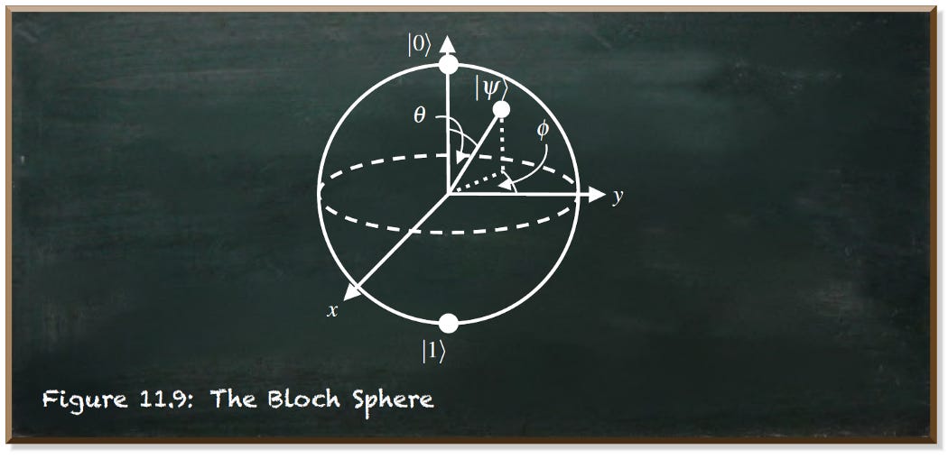
Basically, the quantum state is the vector |𝜓⟩. Its head resides anywhere on the surface of the sphere. The surface also crosses the basis states |0⟩ at the top and |1⟩ at the bottom.

Unfortunately, you'll only see a zero or a one whenever you look at the quantum state. The proximities of the state vector to the basis states denotes the probability of measuring either value. So, you can estimate the proximity by running the circuit repeatedly. But, we're talking about a sphere. There are infinitely many possible quantum states that share the same probabilities. Look at the equator of the sphere, for instance. Any point there has the same distance to the basis states that reside at the poles of the sphere.

To recreate the quantum state, we need to look at the sphere from different angles. This is what we do in quantum state tomography. These are the X, Y, and Z axes. If we have two qubits, there are nine angles: XX, XY, XZ, YX, YY, YZ, ZX, ZY, and ZZ. And, if we have a quantum system that consists of three qubits, there are 27 different angles. So, we have to create 27 versions of our quantum circuit, each representing one perspective.

Fortunately, Qiskit provides a function to create these circuits for us. This function requires the input quantum circuit not to contain any measurements, but we define the qubits to measure when calling the function. Therefore, we set measure=False.

measure = False

from qiskit.ignis.verification.tomography import state_tomography_circuits

st_qcs = state_tomography_circuits(qc, [1,3,5])
print ("There are {} circuits in the list".format(len(st_qcs)))

There are 27 circuits in the list

Even though these circuits are almost the same, their measurements will differ significantly from each other. Therefore, we compute separate modifiers for each of the circuits.

def get_modifiers(qc):
    
    t_qc_sim = transpile(qc, sim)
    noiseless_result = sim.run( assemble(t_qc_sim), shots=shots).result()
    noiseless_counts = sorted_counts(noiseless_result.get_counts())
    
    t_qc = transpile(qc, sim_noisy_jakarta)
    qobj = assemble(t_qc)
    counts = sorted_counts(sim_noisy_jakarta.run(qobj, shots=shots).result().get_counts())
    
    zipped = list(zip(noiseless_counts.values(), counts.values()))
    modifier = list(map(lambda pair: pair[0]/pair[1], zipped))

    print("noisy:     ", counts)
    print("nose-free: ", noiseless_counts)
    
    print("modifier: ", modifier)
    print("\n")
    
    return modifier


modifiers = list(map(get_modifiers, st_qcs))

noisy:      {'000': 125, '001': 120, '010': 136, '011': 123, '100': 115, '101': 125, '110': 132, '111': 148}
nose-free:  {'000': 144, '001': 88, '010': 208, '011': 84, '100': 66, '101': 213, '110': 93, '111': 128}
modifier:  [1.152, 0.7333333333333333, 1.5294117647058822, 0.6829268292682927, 0.5739130434782609, 1.704, 0.7045454545454546, 0.8648648648648649]


noisy:      {'000': 139, '001': 112, '010': 127, '011': 133, '100': 113, '101': 127, '110': 136, '111': 137}
nose-free:  {'000': 162, '001': 88, '010': 233, '011': 33, '100': 29, '101': 213, '110': 118, '111': 148}
modifier:  [1.1654676258992807, 0.7857142857142857, 1.8346456692913387, 0.24812030075187969, 0.25663716814159293, 1.6771653543307086, 0.8676470588235294, 1.0802919708029197]

...

Next, we need to use the modifiers in the state tomography function. I took the original from IBM's source code and changed it. Further, we use OwnResult. This is a class we developed in the previous post. It is a wrapper for the Qiskit Result that allows us to change the counts.

from qiskit.opflow import Zero, One
from qiskit.ignis.verification.tomography import StateTomographyFitter
from qiskit.quantum_info import state_fidelity

# Compute the state tomography based on the st_qcs quantum circuits and the results from those ciricuits
def state_tomo(result, st_qcs, mitigate=False):
    # The expected final state; necessary to determine state tomography fidelity
    target_state = (One^One^Zero).to_matrix()  # DO NOT MODIFY (|q_5,q_3,q_1> = |110>)
    
    own_res = OwnResult(result)
    
    idx = 0
    
    if mitigate:
        for experiment in st_qcs:
            exp_keys = [experiment]
            for key in exp_keys:

                exp = result._get_experiment(key)                
                counts = sorted_counts(result.get_counts(key))
                mitigated = {item[0]: item[1]*modifiers[idx][i] for i, item in enumerate(counts.items())}
                
                #print("original: ", sorted_counts(result.get_counts(key)))
                #print("mitigated: ", sorted_counts(mitigated))
                #print("\n")

                own_res.set_counts(mitigated, key)
    
            idx = idx + 1 
        
    
    # Fit state tomography results
    tomo_fitter = StateTomographyFitter(own_res if mitigate else result, st_qcs)
    rho_fit = tomo_fitter.fit(method='lstsq')
    # Compute fidelity
    fid = state_fidelity(rho_fit, target_state)
    return fid

The function state_tomo takes as parameters the result, the tomography circuits, and a flag whether to mitigate or not. The result must contain the results of all 27 tomography circuits. We start with the definition of the target_state. This is the state that we compare our recreated state with.

The idx variable is a counter for the current circuit. We use it to get the corresponding modifiers. Now, we loop through the circuits, calculate the mitigated counts, and put them into the OwnResult object for the state tomography fitter. Finally, we calculate the fidelity.

So, let's run all these circuits. The noiseless job serves as a comparison.

noisy_job = execute(st_qcs, sim_noisy_jakarta, shots=shots)
noisefree_job = execute(st_qcs, sim, shots=shots)
    
noisy_fid = state_tomo(noisy_job.result(), st_qcs, mitigate=False)
noisefree_fid = state_tomo(noisefree_job.result(), st_qcs, mitigate=False)
mitigated_fid = state_tomo(noisefree_job.result(), st_qcs, mitigate=True)

print('noisy state tomography fidelity = {:.4f} \u00B1 {:.4f}'.format(np.mean([noisy_fid]), np.std([noisy_fid])))
print('noise-free state tomography fidelity = {:.4f} \u00B1 {:.4f}'.format(np.mean([noisefree_fid]), np.std([noisefree_fid])))
print('mitigated state tomography fidelity = {:.4f} \u00B1 {:.4f}'.format(np.mean([mitigated_fid]), np.std([mitigated_fid])))

noisy state tomography fidelity = 0.2161 ± 0.0000
noise-free state tomography fidelity = 0.8513 ± 0.0000
mitigated state tomography fidelity = 0.8317 ± 0.0000

The results show a significant improvement through our mitigation. We almost achieved noise-free fidelity. However, we need to look at these results critically.

We calculated the modifiers using the noise-free results. This is only possible because our circuit is classically simulatable. So, we know the expected outcome. But, of course, taking on all the stress of using a real quantum computer makes only sense for those tasks that classical computers struggle with. But, if we couldn't simulate it classically, we wouldn't be able to calculate the modifiers.

However, our results serve as a proof of concept. We see that quantum measurement mitigation works well and can be used with quantum state tomography.

You're interested in quantum computing and machine learning...

...But you don't know how to get started?