
Solving The Probabilistic Deutsch and Jozsa Quantum Algorithm
Concluding a series of posts on the famous Deutsch and Jozsa quantum algorithm

In the previous post, we developed a probabilistic version of Deutsch and Jozsa’s quantum algorithm.
Deutsch and Jozsa’s original algorithm tells you whether a given function produces constant output (always the same) or balanced output (equal number of zeros and ones). But it assumes the balanced function to be balanced within a specific boundary. If, for instance, the boundary is two (as in Deutsch’s first algorithm), then the algorithm assumes one run to result in 0, and the other result in 1.
When looking at real-world probabilistic systems, such as tossing a coin, this assumption appears unrealistic. You may toss a fair coin three or more times in a row resulting in the same result. Sure, you may doubt whether the coin is fair. The likelihood of having a fair coin decreases with every toss producing the same result. Yet, you can’t conclude that the coin is tricked with certainty.
Our probabilistic version removed this assumption. When the coin is fair with certainty, the algorithm produces the output 0. If the coin might be tricked, the algorithm produces both outputs, 0 and 1. The probability of an output of 1 represents the probability of the coin being fair.
Yet, the algorithm isn’t complete. While it produces different outputs for fair and tricked coins, these outputs are ambiguous. If you have a fair coin, then the algorithm returns always 0. We measure 0 in 100% of the cases. Thus, the probability of measuring 0 represents the probability of having a fair coin — 100%. But when you have a tricked coin, the probability of measuring 1 represents the probability of having a fair coin.
That means, when we measure 1 in 25% of the cases, the chance of having a fair coin is 25%. This becomes problematic when the chance for a fair coin is almost 0. Then, we would almost always measure 0. This implied a tricked coin. But if we always measured 0, it would imply a fair coin.
So, we need to adjust our quantum circuit. Before we start, let’s have a brief look at the first version.
The following figure depicts the circuit with three heads-up tosses.

By contrast, the next circuit shows the circuit with two heads-up tosses and one tails-up toss. The only difference between both circuits is the part of the oracle that represents the respective toss.

The circuit has five parts. First, we put the qubits representing the tosses into superposition. Second, an oracle applies Hadamard gates on qubits representing tails-up tosses. And, it applies controlled-NOT gates on the qubits representing heads-up tosses.
Third, we bring the auxiliary qubit back into state |0⟩ and a triple-controlled-NOT gate calculates the probability of a fair coin given all qubits represent heads-up tosses. Fourth, a series of Z and Hadamard gates followed by another triple-controlled-NOT gate calculates the probability of a fair coin given all qubits represent tails-up tosses.
Fifth, we measure the auxiliary qubit.
If some qubits represent heads-up and others represent tails-up tosses, neither triple-controlled-NOT gate applies, therefore, the auxiliary qubit stays in state |0⟩.
And this is what we aim to change. It should not stay in state |0⟩. It should become |1⟩ instead.
This doesn’t sound too hard, does it? The problem is, however, we must not interfere with either one of the triple-controlled-NOT gates. And this turns out to be a real problem.
Let’s start simple. If we want the auxiliary qubit in state |1⟩, why don’t we remove the NOT gate we apply on the auxiliary qubit just before the triple-controlled-NOT gates?
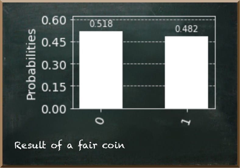
This works pretty well when we have a fair coin. Then, the auxiliary qubit is in state |1⟩.

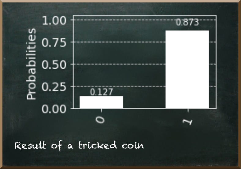
But, when all three tosses are the same, such as heads-up, like in the following figure, then we measure the auxiliary qubit as 1 with the wrong probability. Instead of 12.5%, it is now 87.5%.
Note that inaccuracies are due to the empirical nature of the simulation we use.
Apparently, the solution must consider the qubits that represent the tosses. We must apply a NOT gate on the auxiliary qubit only if all three tosses are in the same state.
So, when all three qubits represent heads-up tosses, they are all in state |−⟩ because the controlled-NOT gates we apply in the oracle perform a phase kickback on them. We could apply Hadamard gates on each of them to bring them into state |1⟩. Then, we apply another triple-controlled-NOT gate. The following Hadamard gates bring them back into |−⟩.

This works pretty well when all three qubits represent heads-up tosses (indicating a tricked coin). Now, the probability of measuring 1 represents the probability of a fair coin.

But it fails once there is a tails-up toss. Then, we don’t measure the qubit as 1 only around 50% of the time.
This is because our newly added triple-controlled-NOT gate applies in this case, too. When you look at the circuit, you see that we applied three Hadamard gates on a qubit representing a tails-up toss. Since the Hadamard gate reverts itself, the first two cancel each other. But the third Hadamard gate puts the qubit into state |+⟩. We also know this state as:

This state is a combination of the basis states |0⟩ and |1⟩. As such, the triple-controlled-NOT gate applies to the |1⟩ part.
OK, maybe we need to apply a different sequence of gates? We can try. But it won’t be successful. The problem is inside our oracle. While we put qubits representing heads-up into state |−⟩ we put qubits representing tails-up into state |1⟩.
These two states are orthogonal to each other. A look at the Bloch Sphere helps here.

We put the qubits representing heads-up and tails-up tosses orthogonal to each other on purpose. It allows us to arrange the qubit states so that the triple-controlled-NOT gates work the way we want them to. We use one triple-controlled-NOT to account for heads-up tosses and one to account for tails-up tosses.
The trick is to put the qubits that represent the correct side (heads or tails) into a state where it has a probability to be measured as 1 of 50%. As a result, each triple-controlled-NOT gate puts the auxiliary qubit only in 1/2³ into state |1⟩. That is the overall probability of a fair coin given the evidence of three tosses with an identical result. But once a single qubit represents the other side, the triple-controlled-NOT does not apply at all anymore because we have put the corresponding qubit into state |0⟩.
We put qubits representing the two sides orthogonal to each other because state |0⟩ is orthogonal to qubit states that exhibit a probability of 50% to measure the qubit as 1 (for instance state |+⟩).
So, while orthogonality helps us to succeed in one calculation it prevents us from doing another. We can’t rearrange the qubits to point into opposite directions easily. It would require us to consider each specific combination of heads-up and tails-up tosses. This would be very cumbersome.
Instead, we add another qubit to represent each toss. And inside our oracle, we apply gates that put the qubits in opposite directions. For instance, we leave qubits representing heads-up in state |0⟩ and qubits representing tails-up into state |1⟩.
Then, we apply another triple-controlled-NOT if either all three qubits represent heads-up or tails-up. Therefore, we measure the auxiliary qubit as 1 with the probability of having a fair coin.
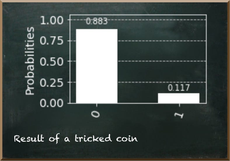
The following figure depicts the final circuit representing an (allegedly tricked) coin that produces heads-up three times in a row.

The results indicate a probability of a fair coin of around 0.125 represented by measuring the qubit as 1.
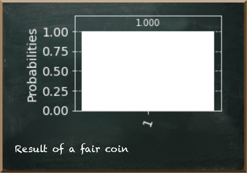
The next figure shows a circuit representing two heads-up tosses and one tails-up toss.

We always measure this circuit as 1 — indicating certainty about having a fair coin.
In this post, we completed our improved version of the Deutsch and Jozsa quantum algorithm.
This final circuit produces plausible results by measuring the auxiliary qubit as 1 representing a fair coin.
Furthermore, this post elaborated on different approaches to solving the given problem — including those that did not solve it. Usually, we focus on the things that work. But I believe that seeing what didn’t work has some value, too. It illustrates the overall process of solving the problem that usually is not as straightforward as we would like it to be. Seeing the approaches that didn’t work may prevent you from doing the same “mistakes” and losing time trying to make something work that doesn’t.